The Definitive Guide to Flow Metrics

In November 2021, Zappts held the Digital Products Month, with several free online lectures and training sessions. One of the topics covered during this month was “How to obtain delivery predictability using flow metrics?”, in a lecture given by Luciano Osorio, Squad Leader, here at the company.

This text was developed based on everything that was explored during the event. For those who want to follow the video, the recording is available below:

To begin, let’s go back a little to the text by our CEO, Rafael Tiba, on “Strategies to reduce the ‘time to market’ of digital products in large corporations”. In this content, besides reducing time to market, Tiba also talked about understanding what happens within our workflow. In today’s conversation, we will talk about these metrics that help us see this flow and be more predictable in our promises and deliveries.

Estimation Methods

To start addressing these metrics, we need to discuss estimation methods for defining project development deadlines. 

• Story Points

One of the most well-known and widely used methods in the market is Story Points. These are a way of saying the size and complexity of what you are developing, as well as pointing out the risk involved in that activity. For example: if an activity is worth five points, but you don’t know much about its subject, increasing the score symbolizes the risk of performing it. 

There is a dynamic used within Story Points to define this estimate, called Planning Poker. Usually, its purpose is to reach a consensus within the team on how many points a given demand is worth.

What are the disadvantages of Story Points?

• It is abstract, as it is not something directly related to the day-to-day of those who receive the project report;
• It doesn’t communicate well with the business;
• There is no direct mapping with effort/deadline;
• It works in the short term, but estimates for demands that will be executed in the distant future become very volatile and revisions will be necessary.

• T-Shirt Sizing

T-Shirt Sizing is a technique used to determine the size of your demand, such as S, M or L. Besides being an even more abstract way than Story Points to make estimates, it brings some difficulties:

• It is confusing. It is not possible to determine, for example, how many S fit into an M;
• There is no relationship with deadlines;
• How to work with demands that don’t fit into S, M or L?;
• It is not possible to measure how many S, M or L fit into the project team’s capacity.

• Hours/Days

Also called ideal hours/days, this is a very common estimation method and has more proximity to the business. It is easier to talk about hours and days. However, just like the methods mentioned above, it has some weaknesses.

• When was the last time you had an ideal day?
• It tries to give a deterministic view of the future. You end up trying to predict something that hasn’t happened yet, where many things can go wrong.
• It excludes queues. In this method, you estimate the time of the work you will perform, without considering the queues it will go through.

• Other techniques

There are countless other techniques that can be used to determine the time and complexity of an activity. For example:

• Guessing, which happens when you don’t know what you’re going to do, so you end up having to guess;
• Pressure, which happens when the volume of pressure exerted on the team makes it assume estimates that are not real;
• Who screams loudest? This happens when someone on the team makes more “noise” to get attention and have their demand met more quickly;
• Deadline determination by the client, or by the boss. Here the team doesn’t even participate in the estimates, someone imposes any deadline and makes it become truth within the project.

Thus, we conclude that estimation methods often fail because they try to determine how much effort is needed to execute the work, often basing it on “feeling” and guesses, and do not consider the time the demand spends in queues. The future does not yet exist and, therefore, it is impossible to determine when these waits will happen.

Flow Metrics

To continue, we need to understand: what is flow?

Flow is the movement and delivery of value to the customer through a process. It occurs from the moment you prepare the materials until the time to enjoy the generated product. For example: the act of making a cake.

Separating the ingredients, mixing them, putting them in the oven and decorating them are acts that make your activity walk through a flow of tasks until delivering value to the customer, which in this case would be tasting the cake.

There are three flow metrics, extremely important to represent how a process works. They are: WIP, Cycle Time and Throughput. 

• Work in Progress (WIP)

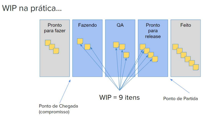
To talk about work in progress, we first need to define what work is in our context. Work is any unit of value for the customer (referred to as items), such as: user story, feature, requirement, improvement, bug, etc.

“In progress” means that the work has been started and is being executed or waiting to be worked on, but has not yet left the system (done).

Thus, WIP is the count of all units of value for the customer that have entered a given process but have not yet left it.

• Cycle Time

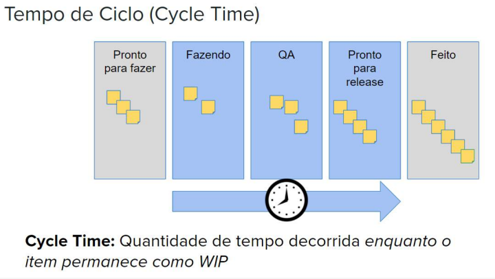
Cycle Time is the time that elapses while the item remains as WIP.

You might be wondering: “Do I need to subtract weekends and holidays?”, “Do I only count business hours?”
And the answer to these questions is: no. Cycle Time is elapsed time, like a stopwatch. It is directly related to how long it takes for you to have the product in the hands of the end customer and, therefore, is closely linked to the event’s theme about Time To Market.

• Throughput

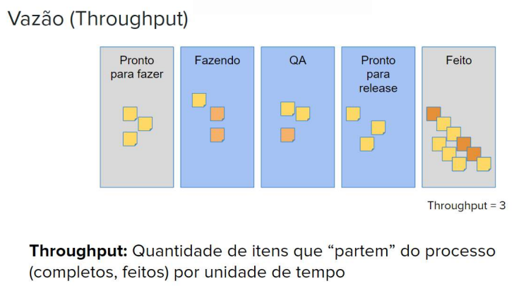
When the work is in the “Done” stage of the entire process, we can measure the throughput of the system.

Thus, we can define Throughput as the number of items that “leave” the process per unit of time.

For example: In a workday it is possible to deliver three new cards.

But why use these metrics and not others?

Because these metrics have predictive power for the customer’s most important question, which is: when will the work be ready?

This is an extremely important and fundamental question for the client from the moment of project negotiation.

Above all, we need to keep in mind that the future does not exist. However, a short-term future, although it cannot be determined, can be predicted with a certain margin of safety. The longer the forecast, the more uncertain it is. For this reason, it is necessary to constantly analyze these metrics and correct forecasts, to ensure that the uncertainty existing in the future does not negatively impact deliveries.

The relationship between flow metrics

The time has come to learn more about the relationship between the metrics presented above and how they determine the answers for the client.

Have you heard of Little’s Law?

Little’s Law states that the higher your WIP, the longer it takes for you to deliver a unit of work, because so many things are happening at the same time that you cannot focus on just one. 

Dr. Little was able to translate this into an equation that says:

“Average Cycle Time = Average WIP / Average Throughput“

Thus, if WIP increases and you maintain the same Throughput, your Cycle Time will also increase. Similarly, if your throughput increases but your work in progress remains the same, cycle time tends to decrease.

This is an empirical relationship. It is much more suitable for studying the past than for predicting the future. This will help you understand how your process is running.

Another thing we need to consider is that this is an average relationship. The average value of each metric does not necessarily represent the current value of each one. So, we need to be very careful not to fall into the temptation of using this equation to “predict the future”, or if we do, to consider the risk assumed in such calculation.

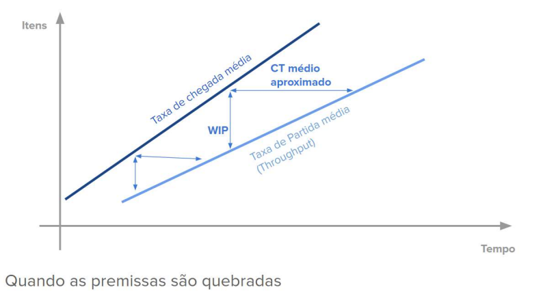
Little’s Law depends on five premises, and it is important to know if they are happening within our flow.

1. The average Arrival Rate of items in your system must be equal, or very close, to the average Departure Rate of the same;
2. All initiated work will be completed and will leave the system;
3. The amount of WIP must be approximately the same at the beginning and end of the time interval chosen for the calculation;
4. The average age of WIP is not increasing or decreasing;

Cycle Time, WIP and Throughput will be measured using consistent units.

When the premises are met, the approximate average Cycle Time is constant.

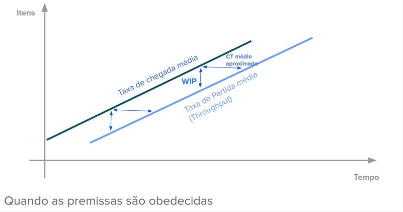
When the premises are broken, it is not possible to determine the approximate average Cycle Time, due to the accumulation of WIPs.

Analytical Tools

Below, we have a Cycle Time chart used to measure a Zappts project. Each of these colored dots is a demand that was delivered. The horizontal lines in this chart, where we have percentages, show that half of the work done in this project was delivered within 6 days. The other half was delivered in a little more than that. For example, looking at the line that points to 85%, we see that most deliveries were made within 19 days.

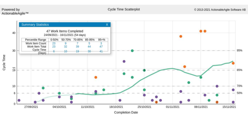
The power of this chart is that, with it, you can predict how cycle time behaves. The more points we have on it, the more we can trust this prediction.

Another way to track Cycle Time is to look at a histogram. This is a chart that counts how many times each cycle time occurred.

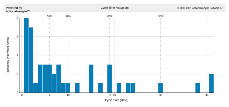
Looking at the chart, we can see that most of the time, Cycle Time was low. Very high times happened, but in smaller quantities. This is exactly what is expected.

Now, observe the Throughput chart below. It is also a histogram, and the concept is the same as the Cycle Time chart — it demonstrates the count of the frequency in which certain throughputs occur.

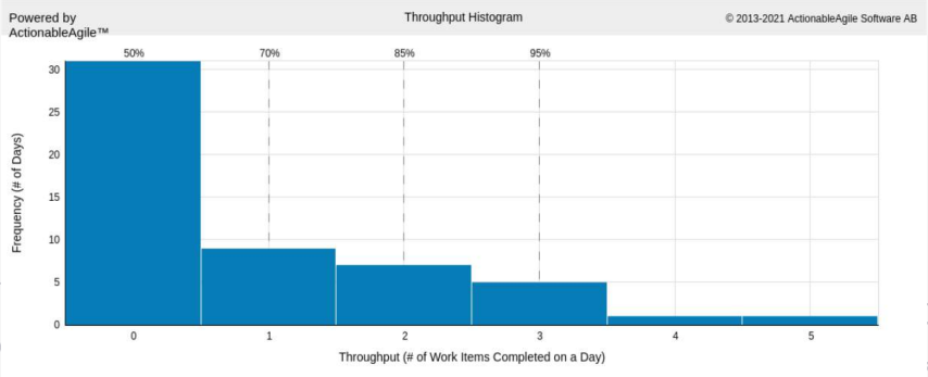
In the case of this project we used as an example, it is possible to see in the chart that we can predict to the client, with 85% chance, that we will deliver two items per day.

In this other chart below, organized by weeks, it is possible to determine how many deliveries were made over time.

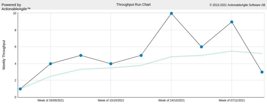
Considering that your sprints last 2 weeks, imagine that your client gives you 15 items to be delivered within this time. Analyzing the type of chart above, it is possible to say whether you can, or cannot, commit to these deliveries.

Back to talking about WIP, the chart below shows how it is possible to evaluate the aging of work in progress.

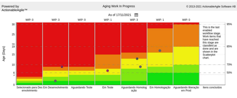
The colored bands correspond to the consumption percentages in each of the phases. If an item is close to the red band early on, there is a high chance it will finish passing through the system with a very high cycle time. Knowing this in advance, it is possible to take actions that resolve this problem.

This is one of the most powerful and important analyses for having control and stability in flow metrics, and requires constant monitoring.

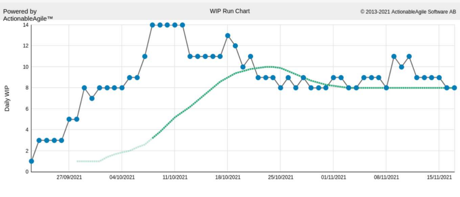
In the chart below, we have the view of work in progress history over time.

Another important and powerful tool we use is Cumulative Flow Tracking. With it, it is possible to analyze Cycle Time by process phase.

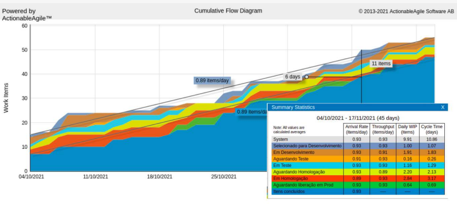
This is an extremely informative chart, and we can extract various information that helps, including, analyzing the stability and predictability premises of Little’s Law.

Each of these colored spaces within the chart represents the number of items we have at each moment, in each of the process phases.

Another analysis method, demonstrated in a histogram, that we can use is Flow Efficiency. It compares the work time of each item with the actual time used until its delivery, and tells what was actually work done and what was waiting time.

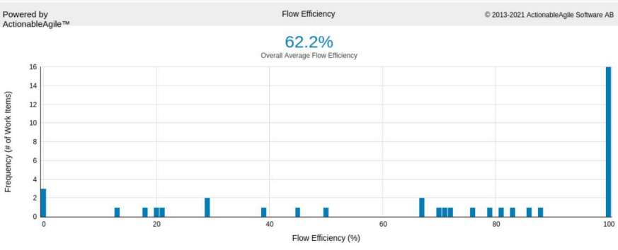
We can observe that, in this example, there are cases where efficiency was 100%, but there are also cases where efficiency was low. In these situations, we need to understand why this happened. 

In cases where your flow efficiency is high (greater than 70%), it is worth investing time in improvements to the work you are actually doing. However, when the efficiency index is low, it is a sign that the item’s waiting time is still long, and it is necessary to work to avoid this.

Our penultimate chart shows us Monte Carlo Analysis. Once you have Little’s Law premises working and a stable process, it is possible to put this data into a statistical model and make predictions. The question that this analysis model answers is: how long will these items take to be ready?

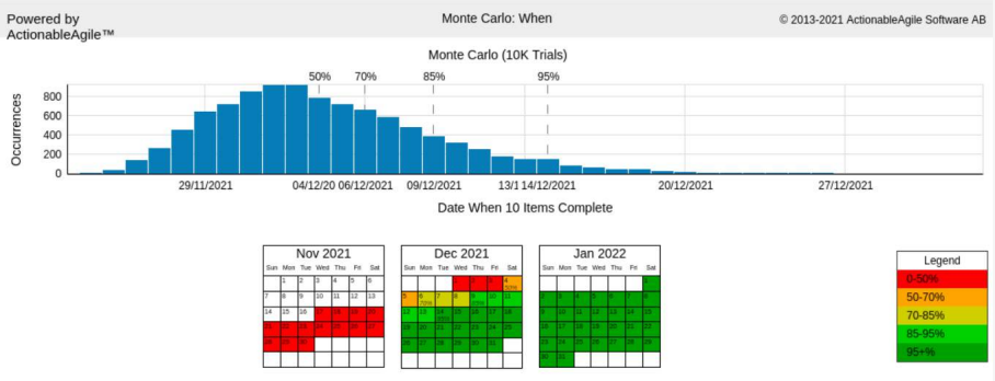
In the chart example, we observe that the items have a 50% chance of being ready on day 04, and more than 95% chance of being ready from day 14 onwards.

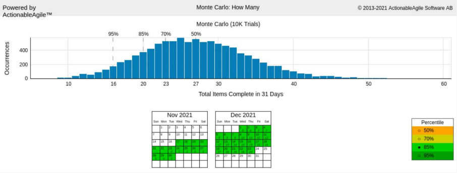
In the chart below, we can see another view of Monte Carlo Analysis. Here, based on our historical information, it is possible to specify the number of items we will have delivered by a certain date, and provide accurate information to the client.

After presenting all these tools for analyzing flow metrics, here comes the question that won’t be silenced:

How much data do I need for all of this to work?

The more data the better, the more history the better. But, statistically speaking, we need to analyze other facts.

• Rule of 5 – The median (the line that separates 50% of the sample below it) of a population will be between the largest and smallest element of a sample of 5 (from that population) with 97.75% certainty. With 5 samples, it is already possible to have a view of where the median is located;
• In a uniform distribution, there is 90% certainty that the 12th value will be between the smallest and largest among the previous 11 values;

These facts tell us that we don’t need an infinity of data to do the analyses. Paraphrasing Douglas W. Hubbard, author of the book How to Measure Anything:

“Having some information is better than having none!”

In the tool we currently use at Zappts, from 10 completed items onwards, as long as they respect Little’s Law premises, it is already possible to perform the analyses we presented.

To finalize, some important considerations:

• Use the same unit of time for all metrics (daily, weekly, biweekly, monthly, etc.);
• Little’s Law is an average relationship and should not be used for predictions;
• The size of items is not the most important!
• Start measuring now!
• Any amount of data is better than no data;
• This presentation is far from exhausting the topic!

About Zappts

Founded in 2014 by Rodrigo Bornholdt and Pablo Augusto, Zappts accelerates the digital transformation of major brands with high-performance teams. Focused on software development, especially in Front-end, UX Design, Quality Assurance, and Cloud Environment Management, it operates in the planning, management, and operation of corporate digital solution development services, environment management, and knowledge transfer through information technology. A reference in creating digital experiences for users, in addition to developing innovative and fast solutions, the company operates on a 100% remote model, with teams distributed across more than 17 states in Brazil.